Annealed Importance Sampling

Computing the exact log-likelihood of an RBM requires the partition function $Z = \sum_{\mathbf{v}, \mathbf{h}} e^{-E(\mathbf{v}, \mathbf{h})}$, which is intractable for large models. Annealed Importance Sampling (AIS) provides a stochastic estimate of $Z$ by interpolating between a tractable reference distribution and the target RBM through a sequence of intermediate distributions at inverse temperatures $0 = \beta_0 < \beta_1 < \ldots < \beta_K = 1$.

This example trains a small RBM on MNIST and then estimates its partition function using both forward AIS (lower bound on $\log Z$) and reverse AIS (upper bound). As the number of interpolating distributions increases, the estimates converge.

import MLDatasets
import Makie
import CairoMakie
import RestrictedBoltzmannMachines as RBMs
using Statistics: mean, std, middle
using ValueHistories: MVHistory
using LogStatFunctions: logmeanexp, logstdexp
using RestrictedBoltzmannMachines: Binary, BinaryRBM, initialize!, pcd!,
    aise, raise, sample_v_from_v

Training

Load MNIST (digit 0 only) and train a small RBM.

Float = Float32
train_x = MLDatasets.MNIST(split = :train)[:].features
train_y = MLDatasets.MNIST(split = :train)[:].targets
train_x = Array{Float}(train_x[:, :, train_y .== 0] .> 0.5)

rbm = BinaryRBM(Float, (28, 28), 128)
initialize!(rbm, train_x)
@time pcd!(rbm, train_x; iters = 10000, batchsize = 128)

 71.917741 seconds (3.15 M allocations: 64.307 GiB, 23.30% gc time, 0.27% compilation time)

Estimating the partition function

We estimate $\log Z$ using aise (forward AIS) and raise (reverse AIS) for increasing numbers of interpolating distributions. Forward AIS provides a stochastic lower bound on $\log Z$, while reverse AIS provides an upper bound. With enough intermediate distributions, both converge to the true value.

First, get equilibrated samples from the model (needed for reverse AIS).

v = train_x[:, :, rand(1:size(train_x, 3), 1000)]
v = sample_v_from_v(rbm, v; steps = 1000)

Now run AIS and reverse AIS with different numbers of interpolating distributions.

nsamples = 100
ndists = [10, 100, 1000, 10_000, 100_000]
R_ais = Vector{Float64}[]
R_rev = Vector{Float64}[]
init = initialize!(Binary(; θ = zero(rbm.visible.θ)), v)

for nbetas in ndists
    push!(
        R_ais,
        @time aise(rbm; nbetas, nsamples, init)
    )
    push!(
        R_rev,
        @time raise(rbm; nbetas, init, v = v[:, :, rand(1:size(v, 3), nsamples)])
    )
end

  3.946689 seconds (5.71 M allocations: 339.397 MiB, 0.69% gc time, 99.19% compilation time)
  0.373265 seconds (490.95 k allocations: 84.301 MiB, 90.12% compilation time)
  1.147000 seconds (12.04 k allocations: 702.855 MiB, 58.78% gc time)
  0.374219 seconds (12.02 k allocations: 730.659 MiB, 4.29% gc time)
  5.454729 seconds (121.84 k allocations: 6.972 GiB, 26.86% gc time)
  5.105647 seconds (121.82 k allocations: 7.262 GiB, 29.07% gc time)
 55.100478 seconds (1.22 M allocations: 69.831 GiB, 26.58% gc time)
 51.882407 seconds (1.22 M allocations: 72.749 GiB, 30.66% gc time)
547.728960 seconds (12.20 M allocations: 698.417 GiB, 26.47% gc time)
492.760250 seconds (12.20 M allocations: 727.621 GiB, 31.39% gc time)

Results

The plot below shows the AIS and reverse AIS estimates as a function of the number of interpolating distributions. Solid lines show the mean estimate (with ±1 std band), while dashed lines show logmeanexp estimates, which are more statistically principled (they correspond to the actual lower/upper bounds on $\log Z$). The red dashed line marks the midpoint of the tightest AIS/reverse-AIS estimates, which serves as our best approximation of the true $\log Z$.

fig = Makie.Figure()
ax = Makie.Axis(
    fig[1, 1], width = 700, height = 400, xscale = log10, xlabel = "interpolating distributions", ylabel = "log(Z)"
)
Makie.band!(
    ax, ndists,
    mean.(R_ais) - std.(R_ais),
    mean.(R_ais) + std.(R_ais);
    color = (:blue, 0.25)
)
Makie.band!(
    ax, ndists,
    mean.(R_rev) - std.(R_rev),
    mean.(R_rev) + std.(R_rev);
    color = (:black, 0.25)
)
Makie.lines!(ax, ndists, mean.(R_ais); color = :blue, label = "AIS")
Makie.lines!(ax, ndists, mean.(R_rev); color = :black, label = "reverse AIS")
Makie.lines!(ax, ndists, logmeanexp.(R_ais); color = :blue, linestyle = :dash)
Makie.lines!(ax, ndists, logmeanexp.(R_rev); color = :black, linestyle = :dash)
Makie.lines!(ax, ndists, -logmeanexp.(-R_rev); color = :orange, linestyle = :dash)
Makie.hlines!(ax, middle(mean(R_ais[end]), mean(R_rev[end])), linestyle = :dash, color = :red, label = "limiting estimate")
Makie.xlims!(extrema(ndists)...)
Makie.axislegend(ax, position = :rb)
Makie.resize_to_layout!(fig)
fig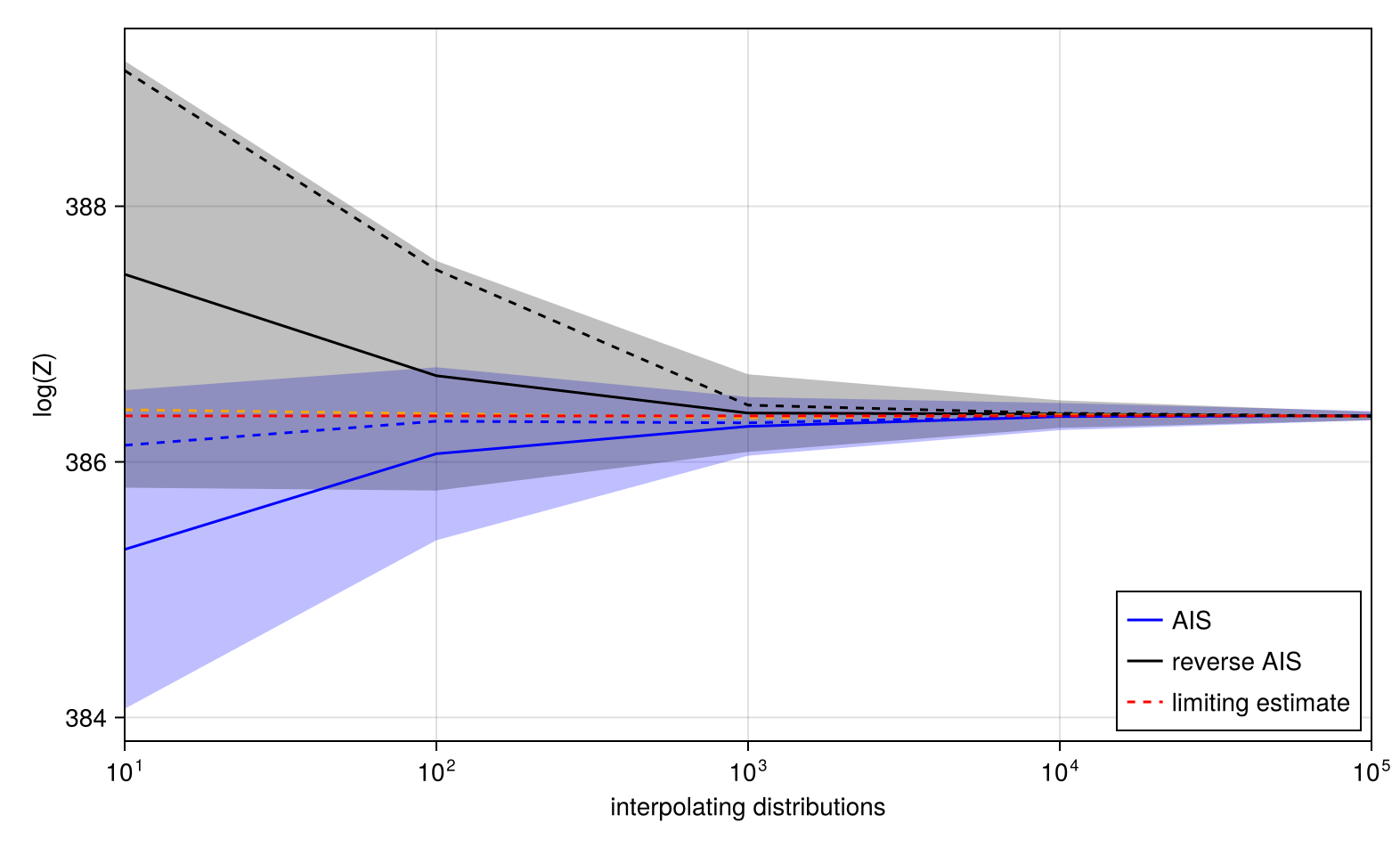

This page was generated using Literate.jl.