dReLU-family layers

The dReLU-family layers (dReLU, pReLU, xReLU, and nsReLU) define continuous hidden units with values in $\mathbb{R}$. Unlike the standard ReLU, they can model asymmetric distributions by using distinct positive and negative branches. dReLU is the most explicit parameterization, pReLU and xReLU use shared-scale parameterizations, and nsReLU fixes that scale to 1. This parameterization was introduced by J. Tubiana et al., "Learning protein constitutive motifs from sequence data".

The potential function is:

\[U(h) = \frac{|\gamma^+|}{2} (h^+)^2 - \theta^+ h^+ + \frac{|\gamma^-|}{2} (h^-)^2 - \theta^- h^-\]

where $h^+ = \max(0, h)$ and $h^- = \min(0, h)$. The parameters $\gamma^+, \gamma^-$ control the curvature (precision) of the positive and negative sides independently, while $\theta^+, \theta^-$ control the location.

In this example we visualize the distribution of dReLU units for different parameter combinations, showing the family of asymmetric shapes also covered by the pReLU, xReLU, and nsReLU variants.

First load the required packages.

import RestrictedBoltzmannMachines as RBMs
import Makie
import CairoMakie

Define the parameter grid.

θps = [-3.0; 3.0]
θns = [-3.0; 3.0]
γps = [0.5; 1.0]
γns = [0.5; 1.0]

Each subplot corresponds to a different $(\theta^+, \theta^-)$ combination. Within each subplot, different curves show different $(\gamma^+, \gamma^-)$ combinations, illustrating how the curvature parameters shape the distribution. Samples are generated per-parameter combination to avoid materializing a large tensor.

fig = Makie.Figure(resolution=(1000, 700))
for (iθp, θp) in enumerate(θps), (iθn, θn) in enumerate(θns)
    ax = Makie.Axis(fig[iθp,iθn], title="θ⁺=$θp, θ⁻=$θn", xlabel="h", ylabel="P(h)")
    for (iγp, γp) in enumerate(γps), (iγn, γn) in enumerate(γns)
        sublayer = RBMs.dReLU(; θp=[θp], θn=[θn], γp=[γp], γn=[γn])
        samples = vec(RBMs.sample_from_inputs(sublayer, zeros(1, 10^4)))
        xrange = range(minimum(samples), maximum(samples), 100)
        pdf_vals = exp.(-only(RBMs.cgfs(sublayer)) .- RBMs.energies(sublayer, reshape(collect(xrange), 1, 100))[1, :])
        Makie.hist!(ax, samples, normalization=:pdf, bins=30, label="γ⁺=$γp, γ⁻=$γn")
        Makie.lines!(ax, collect(xrange), pdf_vals, linewidth=2)
    end
    if iθp == iθn == 1
        Makie.axislegend(ax)
    end
end
fig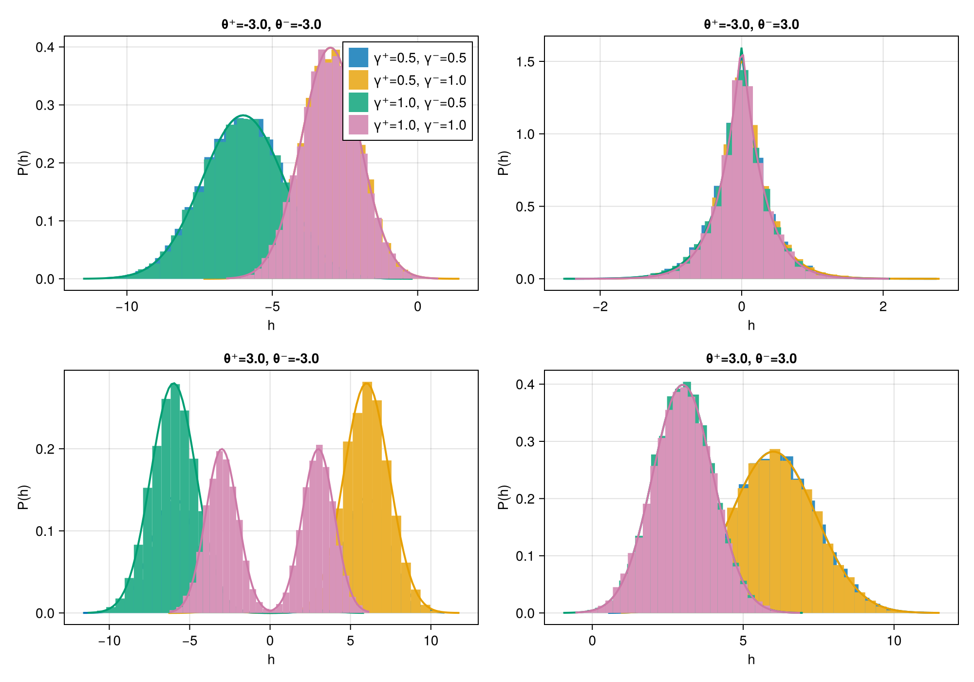

This page was generated using Literate.jl.